Introduction to remiod
intro_remiod.Rmdremiod is acronymed from REference-based Multiple Imputation of Ordinal or Binary variables (Wang and Liu 2022). The purpose of the package is to facilitate the implementation of sensitivity analyses to ordinal/binary response variable with missingness.
Missing data are common in randomised controlled trials (RCTs) and can bias results if not handled appropriately. A statistically valid analysis under the primary missing-data assumptions, usually missing at random (MAR), can be planned, followed by sensitivity analyses under alternative justified assumptions to assess the robustness of results. Reference-based Multiple Imputation (MI) and delta adjustment procedures thus have been developed for analysis under missing-not-at-random (MNAR) assumptions.Tools in this package are developed specifically for reference-based analyses of binary or ordinal responses.
In this vignette, we use the Schizophrenia data which is a part of the remiod package. For more info on this data set, check the help file or visit the following link. The original data is in a long format from a clinical trial, i.e. one row per patient per visit. We first reshape it into a wide format.
data(schizo)

schizow = dcast(schizo, id + tx ~ week, value.var = "imps79o")
colnames(schizow) = c(colnames(schizow)[1:2], paste0("y",colnames(schizow)[-c(1:2)]))

schizow[,colnames(schizow)[-c(1:2)]] = lapply(schizow[,colnames(schizow)[-c(1:2)]],
                                              function(x) factor(x, levels = c("1", "2", "3", "4"), ordered=TRUE))

head(schizow)
#>     id tx y0 y1   y2 y3   y4   y5   y6
#> 1 1103  1  4  2 <NA>  2 <NA> <NA>    2
#> 2 1104  1  4  2 <NA>  1 <NA> <NA>    2
#> 3 1105  1  2  2 <NA>  1 <NA> <NA> <NA>
#> 4 1106  1  2  1 <NA>  1 <NA> <NA>    1
#> 5 1107  0  3  3 <NA>  3 <NA> <NA>    4
#> 6 1108  1  4  4 <NA>  2 <NA> <NA>    3
tx is the treatment variable with 1 being treated and 0 being placebo. y0,y1,…,y6 are the response variables from baseline (visit=0) to visit 6. First, we check the missing pattern of variables in this data using function md_pattern from JointAI.

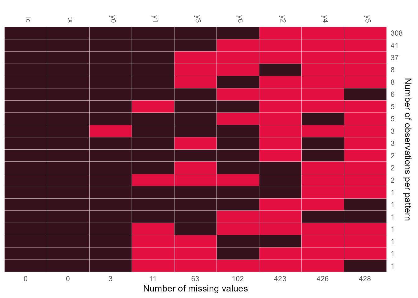
Missing pattern of Schizophrenia data
Figure @ref(fig:missing) indicates there were missing values on the response variable at each visit from the baseline to the last visit. Applying sequential modeling method described by Tang (Tang 2018), remiod function can be set up as follows:
test = remiod(formula = y6 ~ tx + y0 + y1 + y2 + y3 + y4 + y5, data=schizow,
              trtvar = 'tx', algorithm = "jags", method = "MAR",
              n.iter = 0, warn = FALSE, mess = FALSE)
list.models(test)
#>   Order model_formula
#> 1 1     y0 ~ tx
#> 2 2     y1 ~ tx + y0
#> 3 3     y3 ~ tx + y0 + y1
#> 4 4     y2 ~ tx + y0 + y1 + y3
#> 5 5     y4 ~ tx + y0 + y1 + y2 + y3
#> 6 6     y5 ~ tx + y0 + y1 + y2 + y3 + y4
#> 7 7     y6 ~ tx + y0 + y1 + y2 + y3 + y4 + y5
In the default setting, the sequence of models are ordered based on the number of missingness on each variables, which leads to the model on y3 (the number of missing values is 63 as showed in Figure @ref(fig:missing)) preceding to the model on y2 (the number of missing values is 423 as showed in Figure @ref(fig:missing)). In case the sequence of models is expected to follow time order of visits, option model_order = paste0("y",0:5) can be added to specify the model order as y0, y1, y2, y3, y4, and y5, for example:
test_ord = remiod(formula = y6 ~ tx + y0 + y1 + y2 + y3 + y4 + y5, data=schizow,
                  trtvar = 'tx', algorithm = "jags", model_order = paste0("y",0:5),
                  method = "MAR", n.iter = 0, warn = FALSE, mess = FALSE)
list.models(test_ord)
#>   Order model_formula
#> 1 1     y0 ~ tx
#> 2 2     y1 ~ tx + y0
#> 3 3     y2 ~ tx + y0 + y1
#> 4 4     y3 ~ tx + y0 + y1 + y2
#> 5 5     y4 ~ tx + y0 + y1 + y2 + y3
#> 6 6     y5 ~ tx + y0 + y1 + y2 + y3 + y4
#> 7 7     y6 ~ tx + y0 + y1 + y2 + y3 + y4 + y5
Argument method in remiod function is the place to request controlled multiple imputation. method = "MAR" in the example setting above will give imputation based on MAR assumption. Other options include J2R (Jump to Reference), CR (Copy Reference), and delta (delta adjustment).Theoretic aspects of these methods can be found in Tang (2018).
test_j2r = remiod(formula = y6 ~ tx + y0 + y1 + y3, data = schizow, trtvar = 'tx',
                  algorithm = "jags", method = "J2R", ord_cov_dummy = F,
                  n.iter = 20, n.adapt = 10, n.chains = 2, warn = FALSE, mess = FALSE)
names(test_j2r)
#> [1] "mc.mar"     "mi.setting" "mi.data"
Function extract_MIdata can be used to extract an expected number, say M = 5, of imputed data sets following MCMC sampling of remiod. Argument minspace sets the distance, i.e. the number of iterations, between two subsequently selected MCMC samples. If post-processing MCMC samples is required, it can be set through argument mi.setting. For example, mi.setting = list(exclude_chains=2) requests to exclude the second chain of MCMC samples.
extdt = extract_MIdata(object=test_j2r, method="J2R",mi.setting=NULL, M=10, minspace=2)
table(extdt$Imp_)
#>
#>   1   2   3   4   5   6   7   8   9  10
#> 437 437 437 437 437 437 437 437 437 437